Mathematical Transformations of Spatially Balanced Samples
Channeling chaos into balanced, random point density distributions.
library("dplyr")
library("magrittr")
library("sf")
library("glue")
library("spbal")

library("ggplot2")
library("ggExtra")


# set specific seed for reproducability
location_id <- 42
set.seed(location_id)
Introduction
Is Randomness Chaos?
Occasionally, one requires a set of points which are randomly distributed in a given area.
n_samples <- 2^8
x <- runif(n_samples)
y <- runif(n_samples)
data <- data.frame("x" = x, "y" = y)

par(pty = "s")
plot(data, pch = 21, col = "black")
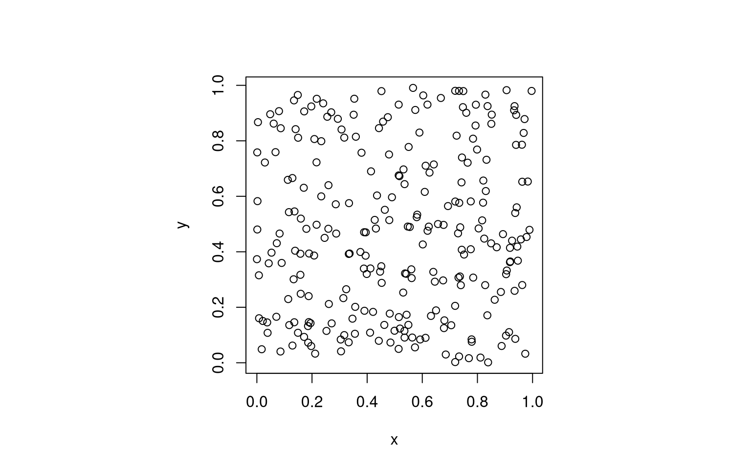
But then, you know, if we are honest, “random” might be a bit too random. Some points come out on top of each other, some areas remain blank, and the corner points are quite far from the center.
Gradually Less Randomness
There are options and choices to modify the randomness to our liking.
(1) Your Inner Circle
First of all, the square layout is not generally useful; imagine another common case where you want to randomly distribute points in a circle. For example, think of sampling data “within a radius or range” of a target location. You could filter the circle within the square.
x0 <- 0.5
y0 <- 0.5
data <- data %>%
  mutate(r = sqrt((x - x0)^2 + (y - y0)^2)) %>%
  filter(r < 0.5) %>%
  select(-r)

par(pty = "s")
plot(data, pch = 21, col = "black")
title(glue::glue("N = {nrow(data)}"))

… but then, your sample size changes (lost about 20% of points, but the number is never exact). So this is not of general use.
Below, I will demonstrate how to create a circular area covered with the defined number of random points, by means of a simple polar coordinate transformation.
(2) Find Your Spatial Balance
A second feature of the initial example random points is that they cluster randomly. This matches the observation that some of the points are close together, whereas other areas are undersampled.
This has disadvantages, e.g. in terms of information theory. If you want to sample information about a geographic area, points proximal to existing measurements provide little extra information (at least if Tobler’s Law holds). Yet, purposefully placing a measurement into “that previously missed open spot” bares the danger of bias, and the cost of potential future oversampling.
What we often desire is spatially balanced sampling, like this:
(3) Choose Your Distribution Pattern
The figure above treats points in all areas of the circle equally.
But then, if you think about it, there are special points in a circular area - obviously, its center.
And in many applications, it is a valid strategy to give points closer to the center a higher chance of being chosen, or to have a sampling pattern that reduces likelihood with distance from center, or just the opposite (i.e. bias towards the rim).
Completely hypothetical example: imagine you want to study the effect of soil pH on plant root growth.
Your experiment starts by measuring pH, and then planting a seed in a specific, central location.
If there is variability in pH, you might want to sample a number of random locations in your study area for averaging.
By prior knowledge, roots spread out all directions, you might know a maximum radius.
However, root density decreases with distance, and the further away from the center, the less likely it is that measured pH will affect your study subject.
A uniform random distribution cannot account for the distance effect: it overrates the samples further away from the center (by including more of them, relatively speaking).
In contrast, the center-weighted sampling strategy can emphasize that data interrelation decreases with distance, making it suitable for any research question about specific points and radially decreasing effect correlation1.

The appropriate distribution of points depends on the (probability density) distribution of the values measured or sampled, and thus ultimately on the research question and subject. Nature creates a variety of distribution patterns, and it might be useful to be able to mimic them with computational sampling. In this tutorial, I will briefly demonstrate, how.
Methods
Functional Programming (a bit)
Throughout this tutorial, I will apply some basic concepts of functional programming. (Really just a tiny, superficial addition, nothing to be excited about.)
As is the habit of my institute, I will use R.
R has strong libraries for spatial analysis (sf, terra), it is moderately good at functional programming (with some severe let-downs, such as cumbersome workarounds for multiple return values), and it is only just catching up on object-oriented programming (e.g. see here).
In this situation, the easiest way I found of implementing a system for basic school geometry are functions like the following wrappers to alleviate some of the unnecessary cumbersome-ness.
# create a two-element point coordinate from a single x and y
create_point <- function (x, y) t(as.matrix(c(x, y), byrows = TRUE, ncol = 2, nrow = 1))

# create a `sf` polygon from a point matrix, via an intermediate data frame
create_polygon <- function(point_matrix, coord_cols = NULL, crs = 31370) {

  if (is.null(coord_cols)) {
    coord_cols <- c("x", "y")
  }

  spatial_df <- as.data.frame(point_matrix) %>%
    setNames(coord_cols) %>%
    sf::st_as_sf(coords = coord_cols, crs = crs)

  return(sf::st_combine(spatial_df) %>% sf::st_cast("POLYGON", warn = FALSE))

}
These functions put in action for another trivial thing we require: a unit square2.
unit_square <- create_polygon(
  rbind(
    create_point(0, 0),
    create_point(0, 1),
    create_point(1, 1),
    create_point(1, 0),
    create_point(0, 0)
  )
)
We will return to it below. The first task will be to get random points within that unit square. Later, we will stretch and morph it to the desired area.
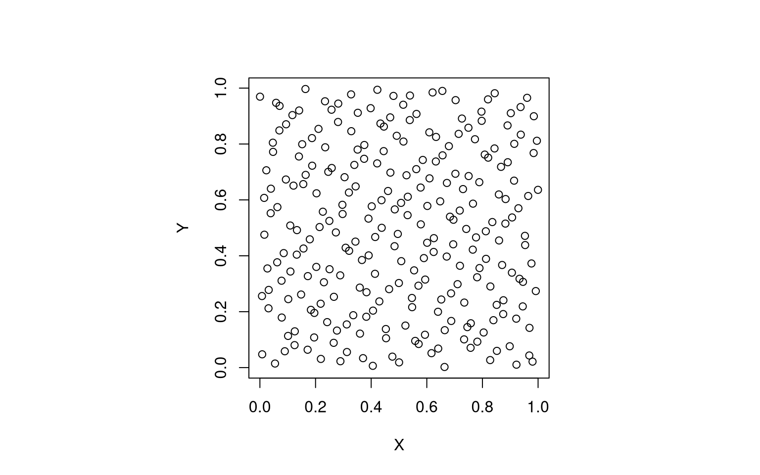
Spatially Balanced Sampling
Balanced Acceptance Sampling (BAS)
This method is a rather recent addition to the toolbox (Robertson et al., 2013). In my own words (which, much like an LLM chatbot, are in fact just the inaccurate transformation of the bunch of cryptic text my neural processing unit has attempted to decipher and categorize during some indefinite training period):
BAS uses mathematical sequences (feel free to read up on the “Halton sequence”) which produce a desired number of quasi-random, multi-dimensional coordinates from a given starting point. That those points are spatially balanced is rather a side-effect. You can add some tweaks and priors to tune the outcome, and the authors claim that the algorithm is computationally efficient.
What else did I need to know?
The library spbal does the job and worked immediately for my simple purpose here.
draw_unit_square_samples <- function(n_samples) {
  result <- spbal::BAS(sf::st_as_sf(unit_square, crs = NA), n = n_samples)
  samples <- result$sample %>% {.[, c("SiteID", "geometry")]}

  return(sf::st_coordinates(samples))

}

n_samples <- 2^8
coords <- draw_unit_square_samples(n_samples)

par(pty = "s")
plot(coords, pch = 21, col = "black")
phi in the paragraphs below.
Generalized Random Tesselation Stratified (GRTS) Sampling
You could equally well use another strategy for generating spatially balanced sample points, like GRTS (Stevens & Olsen, 2003; Stevens & Olsen, 2004).
My leaky internalization procedure has generated the following brief summary of the method: you divide a given area into quadrants of four “pixels” by recursive subdivision, give them an address (which is cleverly solved in a base-four number system), and by their arrangement and the characteristics of the address system you can cleverly retrieve spatially balanced subsets of any size from your base area.
Code example below (Thank you, Floris!). Just note that this particular implementation requires a CRS to be specified; maybe you know a sufficiently generic one.
library("sf")
library("spsurvey")
samples <-
  st_polygon(list(matrix(
    c(0, 0,   1, 0,
      1, 1,   0, 1,
      0, 0    ),
    ncol = 2, byrow = TRUE
  ))) %>%
  st_sfc() %>%
  st_sf(crs = 31370) %>%
  grts(n_base = n_samples) %>%
  {.$sites_base[, c("siteID", "geometry")]}
plot(samples, pch = 21, col = "black")
A desirable feature of spatially balanced sampling is that the sample remains spatially balanced even if you just take a subset from it. If I understood correctly, both BAS and GRTS have this feature, at least if you take a consecutive subset from the start of the series.
This also means that you can append more samples to the end of your set later on.
Transformations
Polar to Cartesian
To this point, we have a unit square and a number of points, evenly distributed throughout it.
But now, a major brain twister: imagine the sides of that unit square to be not x and y, as we are commonly used to, but an angle (direction) and a radius (distance).
This is easiest to understand in tabular form:
just take the values we have, and rename them to phi and r:
as_tibble(coords) %>%
  setNames(c("phi", "r")) %>%
  head(5) %>%
  knitr::kable()
| phi | r |
|---|---|
| 0.2301 | 0.3054 |
| 0.7301 | 0.6387 |
| 0.4801 | 0.9721 |
| 0.9801 | 0.0214 |
| 0.0270 | 0.3548 |
Because, to be honest, I have tricked you from the beginning: The unit square was not a unit square in Cartesian space, but is a unit square in Polar coordinates.
If you are afraid of polar coordinates, fret not, because the next thing we will do is to transform them back to our well-known x and y.
Though, one more thing: To be able to do more stretching and bending below, we will also prepare a tiny “transformation” algorithm (apply_trafo).
No worries about that either: we start with the “identity” transform 3, and later try our more (or less) crazy stuff.
identity_trafo <- function(x) x

# apply a transformation to a df of coordinates
apply_trafo <- function(coord, trafo_fcn = identity_trafo, scale = 1) {

  # we simply transform
  coord <- trafo_fcn(coord)

  # scale the transformed coordinates back to the desired range (usually the unit interval)
  return(scale * coord / trafo_fcn(1.))
}
Functional programming basics:
the function apply_trafo takes a function as an input argument.
It then applies it, but also does some more stuff (here: scaling).
You could say that we just invented a simple, dynamic “wrapper”.
Finally, we get our x and y back as follows:
target_radius = 10 # m
angle_range = 2 * pi # radians
phi <- coords[, 1]
r <- coords[, 2]
phi_transformed <- apply_trafo(phi, scale = angle_range)
r_transformed <- apply_trafo(r, scale = target_radius)
convert_polar_to_cartesian <- function(distance, direction, rotation_rad = 0) {
# convert to x/y
x <- distance * cos(direction + rotation_rad)
y <- distance * sin(direction + rotation_rad)
return(data.frame("x" = x, "y" = y))
}
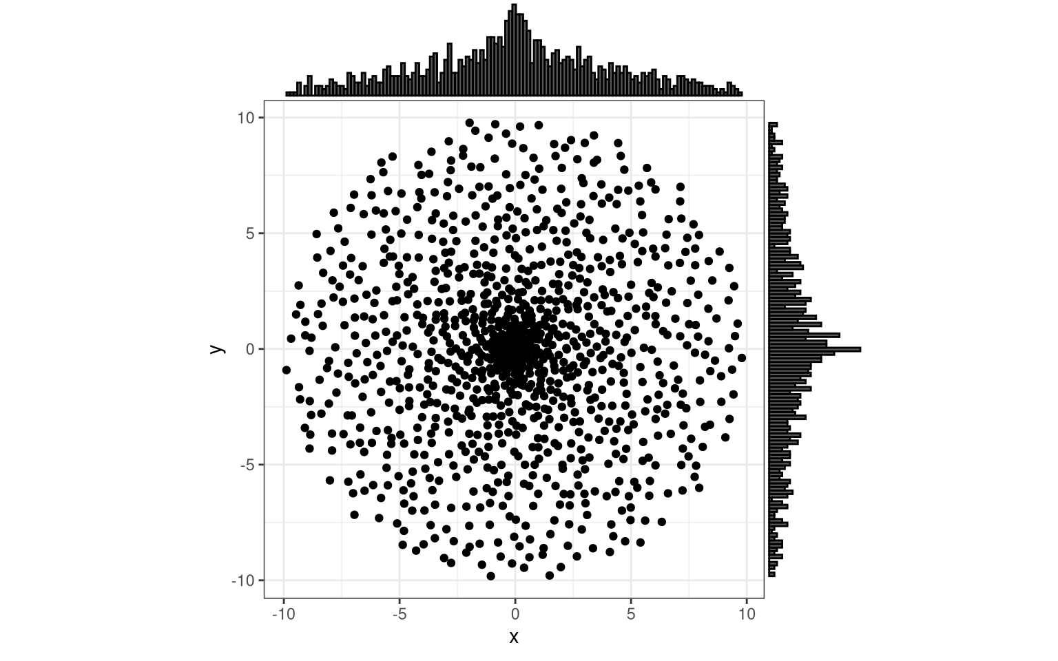
data <- convert_polar_to_cartesian(r_transformed, phi_transformed)
par(pty = "s")
plot(data, pch = 21, col = "black")
title(glue::glue("{nrow(data)} points, spatially balanced in a circle -- or not?"))
![]()
Does the outcome surprise you?
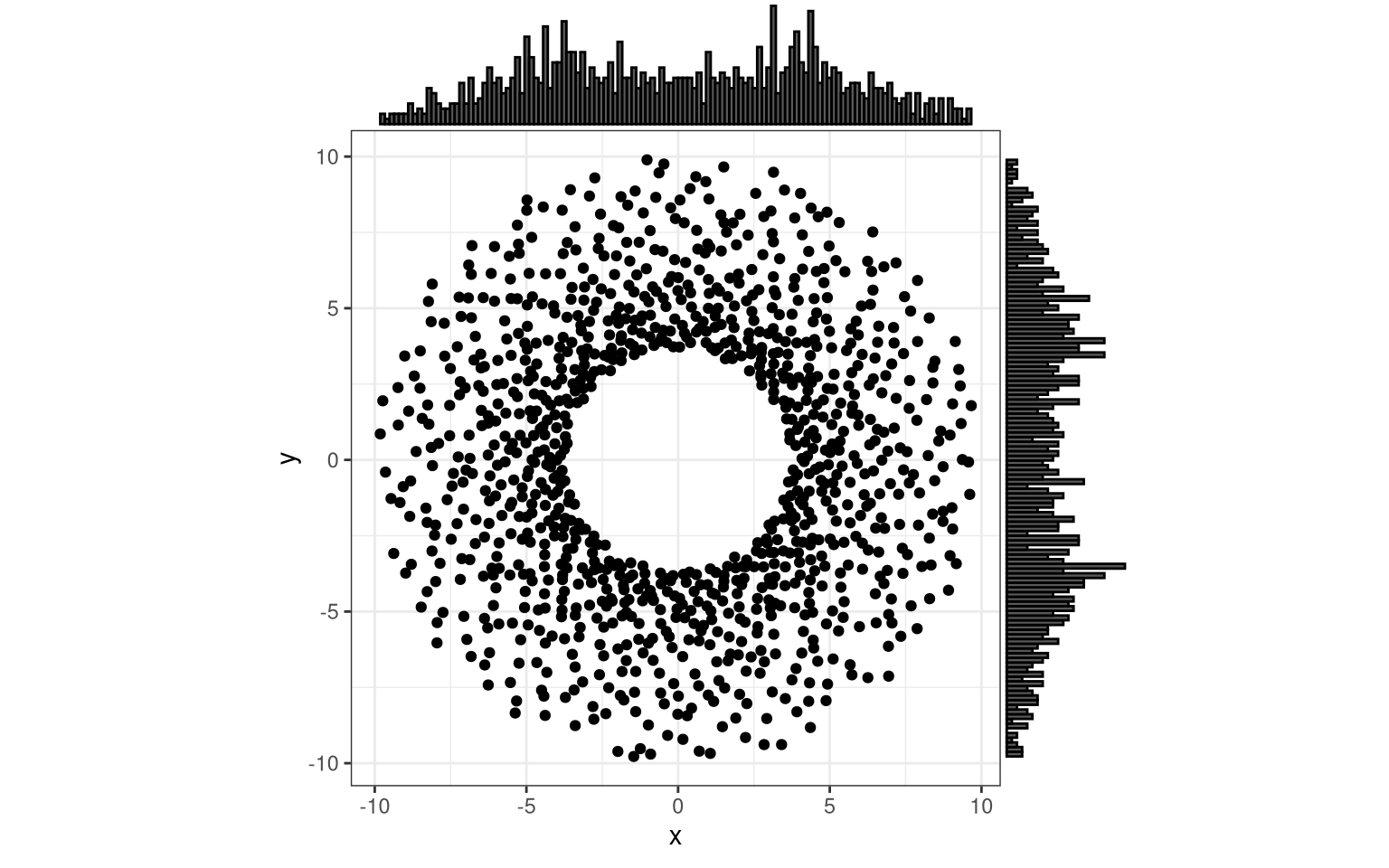
Spatial Balance - in a Weird Way
Note how the sample is still spatially balanced, but in a way that one might not have expected:
- At each distance from the center, there is an equal chance of finding a point.
- Across all directions, points are uniformly distributed (i.e. everywhere the same chance to see points).
However, point density (the chance of finding a point in a given “pixel” window), is not homogeneous. Close to the center, it is high, but it reduces towards the edges of our circle. Logical, if you think about it: the orbits close to the center are much shorter, yet they house equally many points as the distant orbits.
This outcome might be fine in some situations (e.g. where there is a radial component to the correlation structure or physical measurement; think of sources and sinks and limited diffusion), but undesired in others (e.g. repeated measurements in perfectly homogeneous mixtures or systems).
Finding the Inverse Transformation
If we want to go for homogeneous point density in our circle, we need to nullify the tendency of our points to cluster round the center. Even if you did pay attention in highschool maths, you might not immediately know which of the usual suspect functions counteract the “orbit effect”, and in which direction to apply it. Exponential? Gaussian? Polynomial? Hyperbolical? Just saying something.
To support my own sparse maths memory, I like to trial-and-error my way out with functional programming. What helps me are concise functions to test the same procedure over and over with altering input arguments (also functions); I often iterate over all the usual suspects.
# just the same procedure as above, with more points
test_trafos <- function(trafo_r = identity_trafo, trafo_phi = identity_trafo, n = 2^10) {
coords <- draw_unit_square_samples(n)
r <- apply_trafo(coords[, 2], trafo_r, scale = target_radius)
phi <- apply_trafo(coords[, 1], trafo_phi, scale = angle_range)
data <- convert_polar_to_cartesian(r, phi)
return(data)
}
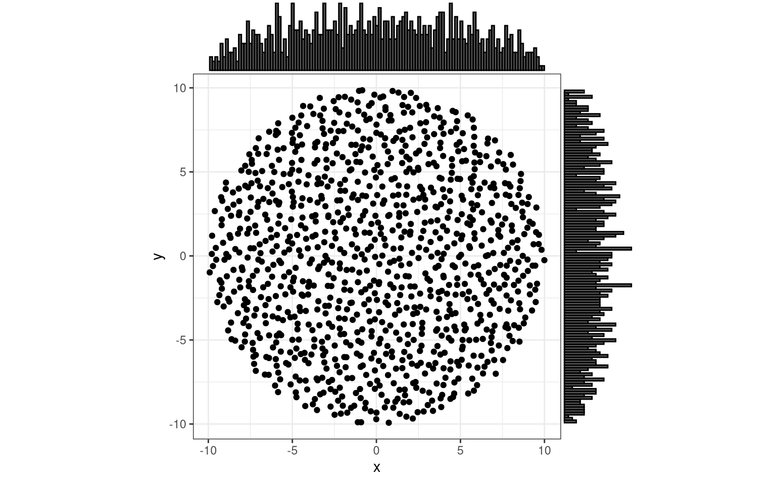
margin_plot <- function(data) {
h <- ggplot(data, aes(x = x, y = y)) +
geom_point() +
theme_bw() +
coord_fixed(ratio = 1)
ggMarginal(h, type = "histogram", bins = 2^7)
}
# plot the distribution, using "identity", i.e. the re-transformed radii
margin_plot(test_trafos())
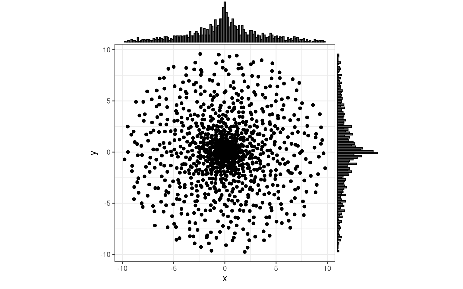
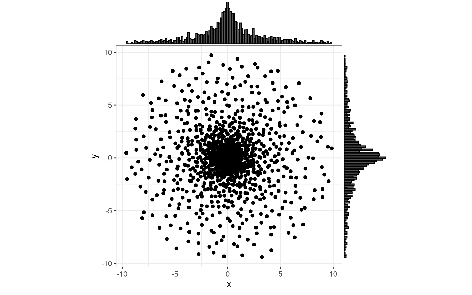
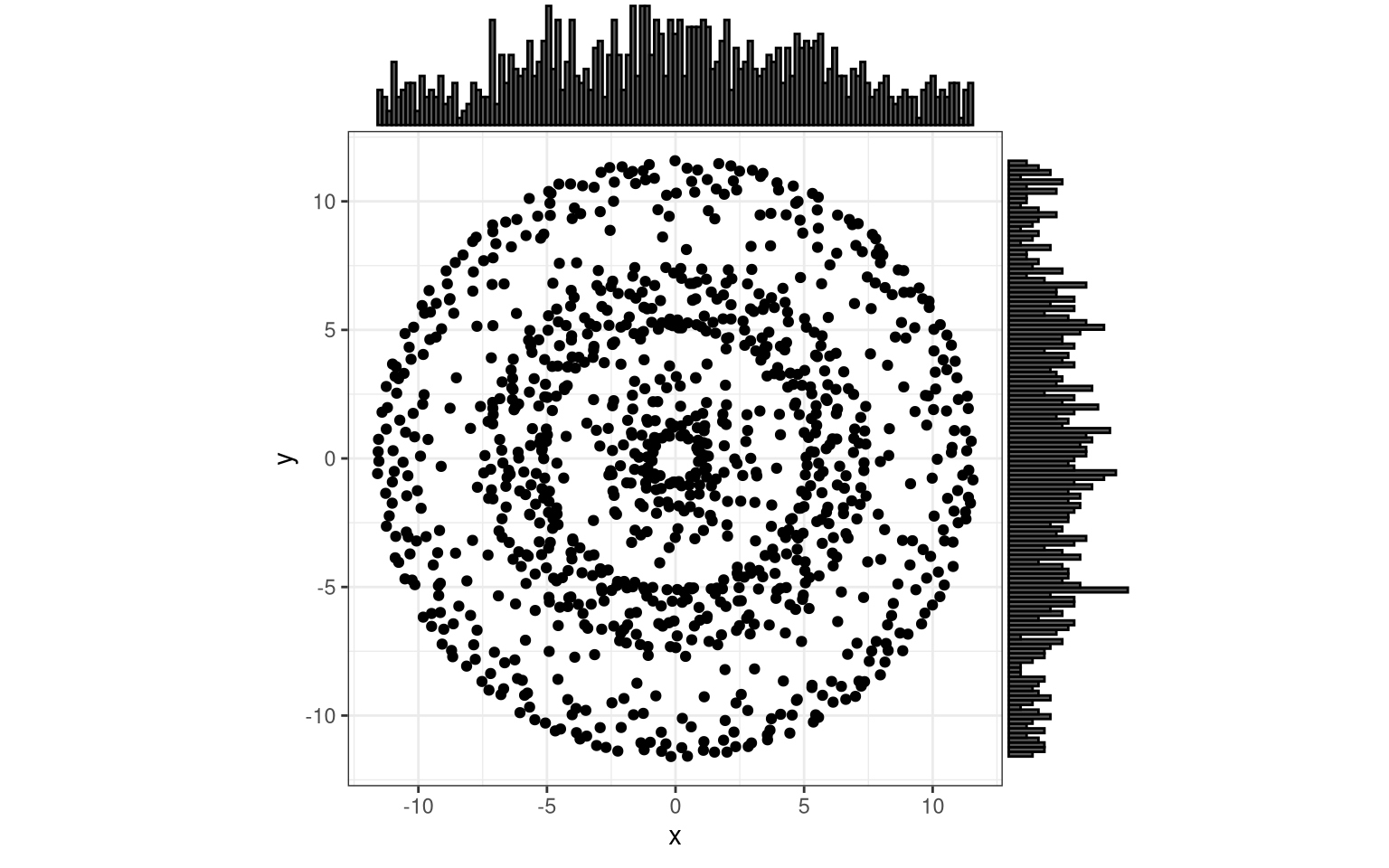
You can inverse the “center-heavy” distribution. Admitted, I trial-errored this initially, but the result makes sense:
- the surface of a circle increases with \(\sim r^2\) (surface, because remember, we want to homogenize density)
- square root is the inverse operation
So to get the distribution uniform, we apply the square root. (The skalar \(\pi\) in \(A = \pi r^2\) does not matter because of a distance normalization hidden in the wrapper above.)
inverse_radial <- function(x) sqrt(x)
par(pty = "s")
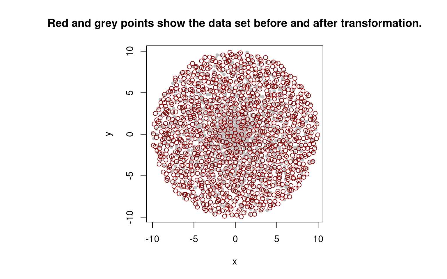
plot(test_trafos(), pch = 20, col = "grey") # for comparison: original points
points(test_trafos(trafo_r = inverse_radial), col = "darkred") # transformed points
title("Red and grey points show the data set before and after transformation.")
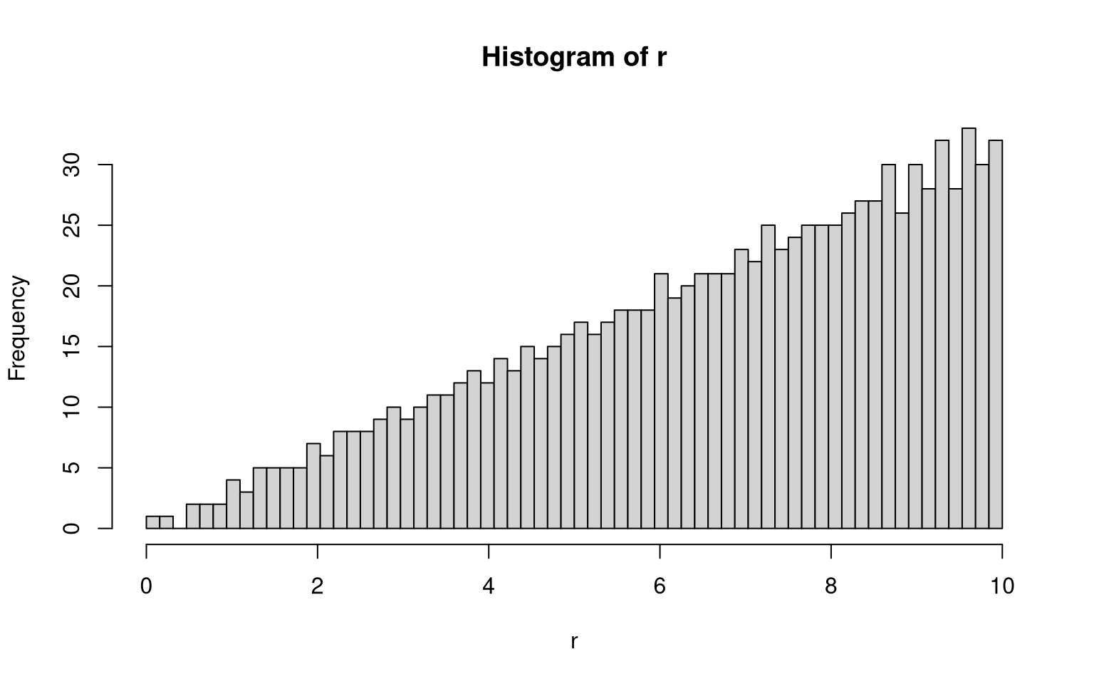
You can also see this on the histogram of radii:
coords <- draw_unit_square_samples(2^10)
r <- apply_trafo(coords[, 2], inverse_radial, scale = target_radius)

hist(r, breaks = seq(0, target_radius, length.out = 2^6+1))
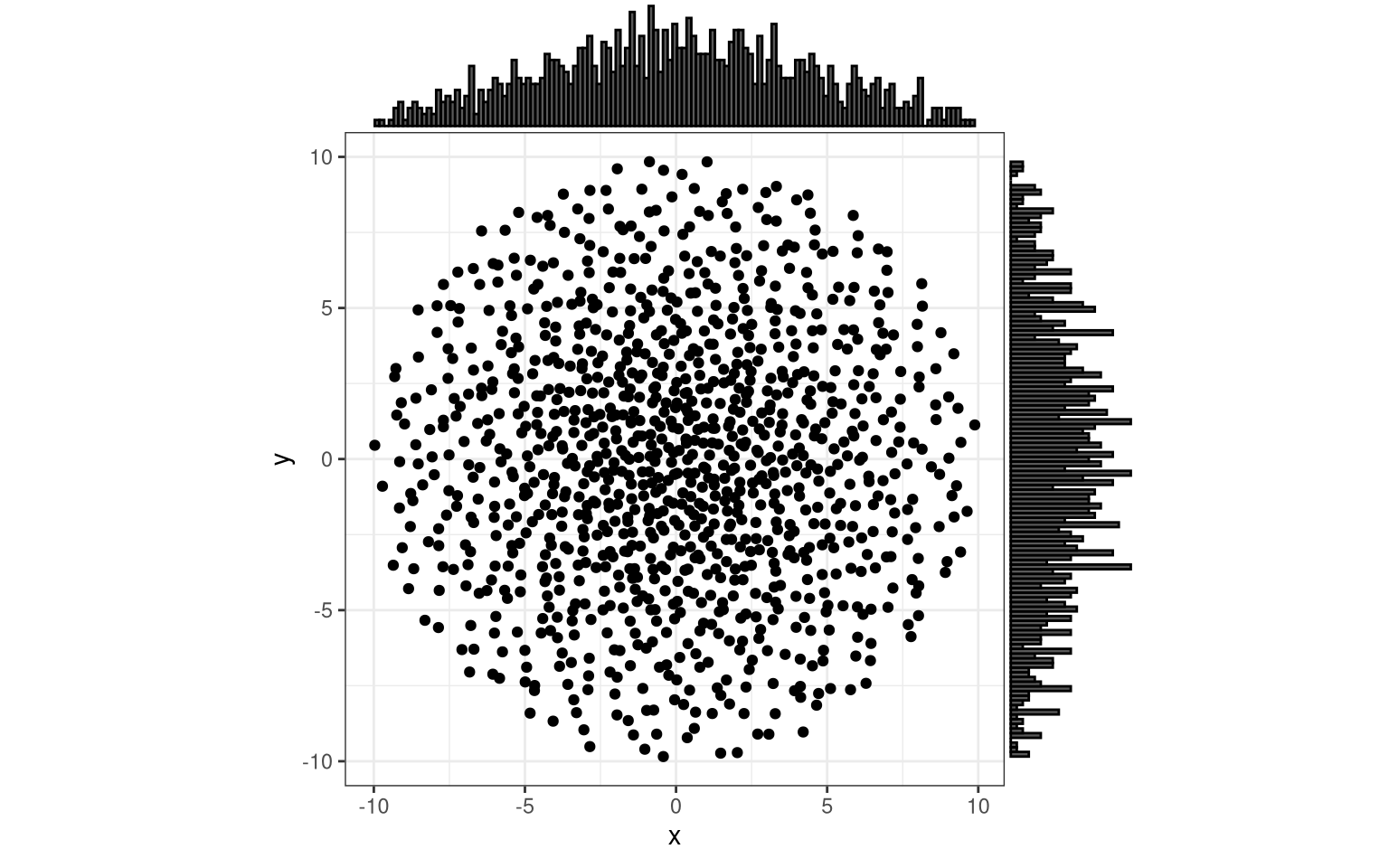
Let us apply this to give the test_trafos() function above the option to uniformize prior to transformation.
test_unif <- function(trafo_r, ..., uniformize = TRUE) {

  if (uniformize) {
    trafo_r_unif <- function (x) trafo_r(sqrt(x))
  } else {
    trafo_r_unif <- trafo_r
  }

  data <- test_trafos(trafo_r = trafo_r_unif, ...)

  return(data)
}

# trying the identity trafo
data <- test_unif(trafo_r = identity_trafo, n = 2^10)
margin_plot(data)
Nice, functional programming with the “ellipsis” (the “...” in the function signature).
Our test_trafos gained the extra capability of returning a spatially balanced distribution of points in a circle.
Find Your Own Transformation
With these tools at hand, you can easily distribute the points in any radial pattern you like.
One more wrapper function to wrap this whole thing up:
trial <- function(test_trafo) {
  margin_plot(
    test_unif(
      trafo_r = test_trafo,
      n = 2^10,
      uniformize = TRUE
    )
  )
}
And, here you go, have fun:
trial(function(x) tan(x))
trial(function(x) exp(x^2))
Oh… Wait… What happened here?
Ah, yes!
1 = exp(0), and should be shifted down by one.
trial(function(x) exp(x^2)-1)
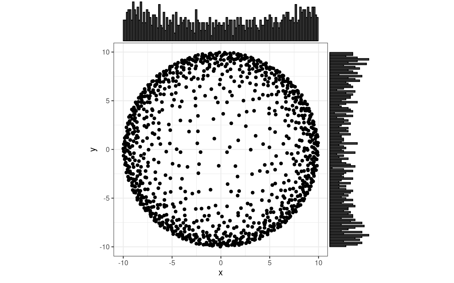
You could move more density to the borders, giving bowl-shaped (marginal) distributions.
trial( function(x) atan(4*x) )
You can try to approximate a Gaussian, and I am sure there is an analytical way to represent it in polar coordinates (see also). However, if you need a Gaussian, you could also directly go to the 2D Gauss function, without the need for the polar-to-cartesian transformation trick.
sigma <- 0.5
gauss <- function(r) r*exp((r^2)/(2*sigma^2))
# xi <- seq(0., 1., length.out = 101)
# plot(xi, gauss(xi))
trial( gauss )
You can even get periodic, concentric bands of points, and as you would suspect these require trigonometric functions and/or complex numbers.
trial( function(x) x + 0.2 * sin(16 * x) )
Admittedly, my imagination falls short of finding concrete, real-life examples for these special distribution patterns. Nonetheless, I am fascinated by the computational capability of producing them. And if you encounter basically any more or less regular spatial distribution, you now possess the basic tooling and can take these ideas and concepts further, for your own purposes.
Summary
In this tutorial, I assembled several simple tools to randomly distribute a given number of points in a circular area with homogeneous point density. This originated from the practical need to identify random points in not perfectly random places. The procedure draws from existing, widely acknowledged methods; no claim of novelty from my side.
On the one hand, there are algorithms for spatially balanced sampling, and I copy-pasted code to use the standard toolboxes for GRTS and BAS. On the other hand, a series of mathematical operations can transform polar coordinates of balanced samples into cartesian space, then revert the associated distribution patterns, and then go wild by superimposing new distribution schemes.
A major philosophical question remains, and I will leave it up to you to make up your mind about it. After all these choices and adjustments, do you think that we can still say with confidence that distribution we created is random?
As always, I hope this is useful for someone, and I appreciate your feedback and additions.
References and Notes
Robertson B.L., Brown J.A., McDonald T. & Jaksons P. (2013). BAS: Balanced Acceptance Sampling of Natural Resources. Biometrics 69 (3): 776–784. https://doi.org/10.1111/biom.12059.
Stevens D.L. & Olsen A.R. (2003). Variance estimation for spatially balanced samples of environmental resources. Environmetrics 14 (6): 593–610. https://doi.org/10.1002/env.606.
Stevens D.L. & Olsen A.R. (2004). Spatially Balanced Sampling of Natural Resources. Journal of the American Statistical Association 99 (465): 262–278. https://doi.org/10.1198/016214504000000250.
-
Conversely, probability might also increase with distance. An ad hoc hypothetical example which comes to my mind are territorial, competitive species and the chance of finding a conspecific as a function of distance from a known location. ↩︎
-
“Unit” indicates that the dimension extent of all relevant dimensions is one (i.e. one in the chosen units). For example, a unit square spans the area from points (0, 0) to point (1, 1), and a unit circle has a radius of 1 and goes 1 full round. ↩︎
-
“Identity” is just maths-speak for something that is identical on both sides of an equation, such as a function / projection / transformation for which the output always equals the input (take
y = x). ↩︎